Imagine booking a GPU for a long training run. A few hours in, you discover that the sequence length barely fits in memory. Or perhaps the model fits perfectly, but each update takes so long that the planned token budget is out of reach. Neither problem requires a long run to discover. You would much rather learn about it in the first few minutes.
That is the point of a scaling experiment. Don’t ask a small run to predict the final model. Ask it to remove one expensive uncertainty. A useful probe has a specific question, a controlled change and a measurement that can actually answer it. The hard part is knowing what the result doesn’t tell us.
A cheap question before an expensive one
The training loop established what an update means. Before scaling those updates, there are several different things worth checking, and they deserve different experiments.
A smoke test asks whether a configuration can execute a few updates without an immediate failure. A fixed-batch overfit test asks whether the system can learn a deliberately repeated example. A stability probe lets successive batches flow through the model and watches what happens to loss and gradients over a longer stretch. These tests get progressively closer to ordinary training, but they are not interchangeable.
The repository makes that progression concrete. Its smoke configuration specifies 20 updates at batch size 1 and context length 128. The overfit configuration repeats a batch for up to 2,000 updates. The stability configuration instead specifies 1,000 updates on successive batches, with accumulation, warmup and cosine decay.
Those are defined experimental recipes, not three verified outcomes. The YAML tells us what we can attempt. Only a corresponding run manifest and metrics can tell us what actually happened.
How big is a batch, really?
Suppose one microbatch fits comfortably on the GPU. Is that enough to choose the training batch? Not quite. The model updates its weights only after all accumulated microbatches have contributed their gradients.
For this trainer, the nominal number of training tokens processed per successful update is
where is the number of sequences per microbatch, is their length and is the number of gradient-accumulation passes. In the checked-in stability recipe, , and . That means 512 nominal tokens per update, even though each forward pass sees only 128 tokens. The CLI reports this quantity explicitly.
Why not simply make four times larger? Because those choices place different demands on the machine. Increasing the physical microbatch retains more activations at once. Accumulation keeps the microbatch smaller, at the cost of additional forward and backward passes before an optimizer step. In Kimi K3, there is another subtlety: Quantile Balancing updates routing state on each training forward, so four microbatches are not guaranteed to be mathematically identical to one concatenated batch. The trainer documents this distinction.
Context length changes the experiment
The sequence length looks like another multiplier in that equation, but changing it does more than add tokens. A longer context changes which earlier tokens the model can use for each prediction. It also changes activation memory and the work performed by the attention layers. An experiment at can therefore tell us that a short-context configuration runs, not that will be equally efficient or even fit.
There is also an implementation constraint. For chunkwise or fused KDA, the training entry point requires sequence lengths divisible by the configured KDA chunk size. In the scaled model configuration, that chunk size is 64. A context sweep must respect this boundary rather than treating every integer as a valid candidate.
A useful context probe therefore measures two separate things: whether the selected configuration fits within memory, and how many training tokens per second it processes after startup overhead. Neither observation, on its own, shows that the longer context improves final language-model quality.
Change one knob, or learn nothing
Now suppose one trial has a lower loss than another. Was the learning rate better? It is tempting to say yes, especially when GPU time is scarce. But if the second trial also changes batch size, context and number of tokens processed, the comparison cannot isolate the learning rate.
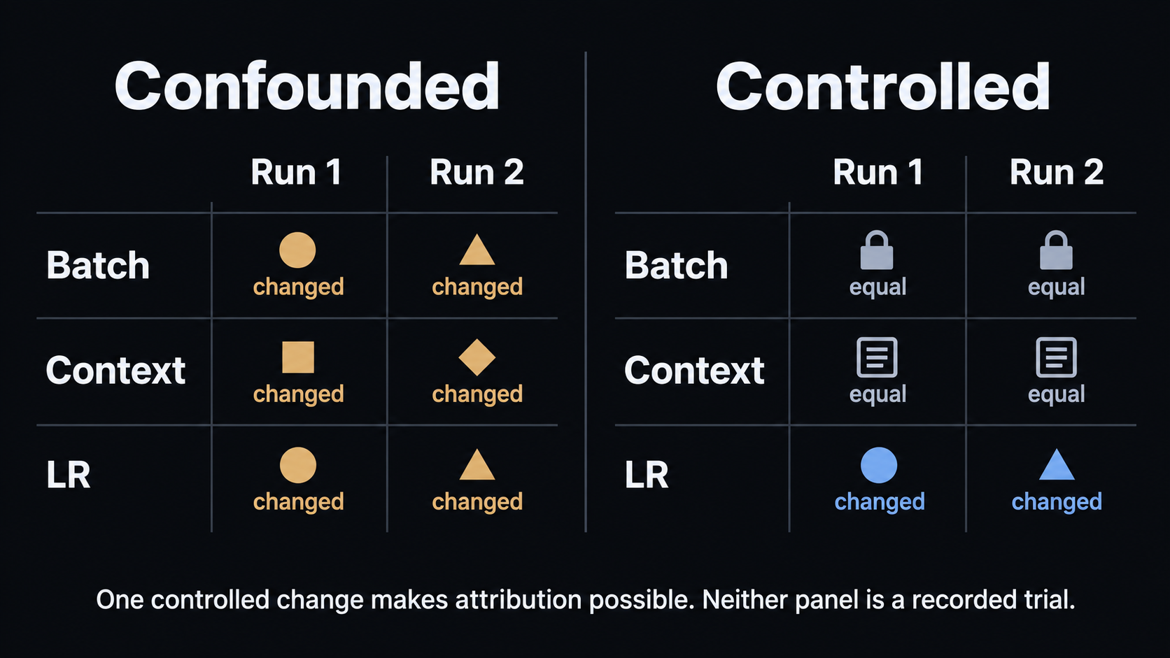
For a learning-rate probe, hold the model, tokenizer, data split, physical batch, context, accumulation, optimizer recipe and evaluation method fixed. Start from comparable initialization and optimizer states. Change the learning rate, then examine early loss, gradient norms, non-finite events and any skipped updates over the same token budget. The trainer exposes learning rate, warmup and decay as explicit configuration values, making the proposed comparison reproducible in principle.
Even this is a limited result. A rate that looks stable over a short window may misbehave later. A rate that reduces training loss quickly may give worse validation loss after enough tokens. And one seed gives a noisier answer than repeated runs. A short probe is good at ruling out obvious trouble, not declaring a universal winner.
The same discipline applies to batch or context comparisons. Vary the quantity under study, keep the other knobs fixed, and record enough metadata to explain any unavoidable differences. A comparison is only as useful as its controls.
Throughput has two clocks
One setting can perform excellent training updates and still make a poor long-run choice. Perhaps it saves checkpoints slowly, or evaluation occupies a substantial fraction of elapsed time. We need to distinguish the speed of the learning work from the speed of the entire session.
The monitor records training tokens per second over training windows and session-wide tokens per second over elapsed time. Training windows include batch retrieval and the training computation but exclude intervening evaluation, checkpointing and reporting. The integration test for timing checks that distinction with a controlled clock. It is a test of metric accounting, not a GPU benchmark.
A short warmup also matters. Early updates can include initialization and other one-off costs. The run summarizer can exclude complete logging windows up to a chosen step and compute a time-weighted steady training rate. It separately reports session-wall throughput and memory peaks. Comparing one run’s warmup-heavy average to another run’s steady rate would make the faster configuration look slower for the wrong reason.
What earns the right to scale?
A small experiment earns a narrow conclusion. A successful smoke test supports basic execution under its particular conditions. A fixed-batch overfit supports the ability to learn that repeated example. A controlled throughput probe supports a speed comparison on the hardware and software it actually used. None of these automatically predicts an uninterrupted, stable pretraining run.
The pilot recipe and pretraining recipe specify a larger configuration: 32 sequences of length 1,024 per update, with BF16 precision and a shared learning-rate schedule. They show the chosen configuration recorded in the repository, not a published batch/context/LR ablation or proof that those values were best. The currently inspected repository snapshot does not include the original logs needed to reconstruct that selection.
So the decision to scale is not “the small run went well.” It is more precise: we have eliminated immediate execution problems, we can state the cost of a candidate configuration, and we know which uncertainties still require a longer experiment. The next task is to test those assumptions on the target GPU itself, with memory headroom, profiling and recovery checks. That is where GPU Qualification begins.