Imagine two parts of a language model. One is a large matrix that turns a token’s representation into a new one. The other is a tiny normalization scale that adjusts the strength of a signal. Both receive gradients. But should we ask them to change in exactly the same way?
A gradient tells us how the loss responds to a small change. It doesn’t tell us how to package that change into a useful, numerically safe update. In this project, that decision becomes a hybrid Muon + AdamW recipe, with a learning-rate schedule and a few carefully placed safeguards. The interesting question isn’t which optimizer has the more impressive name. It’s which structure we want each update to respect.
Why treat a matrix differently?
Picture a matrix as a collection of directions. Each row contributes to how an input representation is transformed. If several directions in a proposed update point almost the same way, changing all of them together may concentrate the update in a narrow part of the matrix’s space.
AdamW treats each parameter coordinate using its own history of gradients and squared gradients, then applies decoupled weight decay. That’s a sensible general-purpose rule, particularly for parameters without a meaningful matrix geometry.
Muon takes another approach for selected hidden matrices. It first builds an update using momentum and optional Nesterov lookahead. Then it approximately orthogonalizes the matrix update: the goal is to make its directions less redundant, rather than simply normalize each individual entry. It uses a short Newton–Schulz iteration to approximate this matrix transformation, without computing a full singular-value decomposition.
The distinction matters more than the formula, but the implementation’s scaling rule is worth seeing:
Here is the momentum-based update before orthogonalization, and are the matrix dimensions, is the learning rate, and denotes the approximate Newton–Schulz transformation. Weight decay is applied separately. The actual optimizer uses the Moonlight shape factor and a five-iteration polynomial by default, with its upstream attribution recorded in the repository.
This is approximate orthogonalization, not a guarantee that every resulting singular value is exactly one. Nor does the existence of a different update geometry establish that Muon trains this particular model better than AdamW. That is a comparison an experiment would have to answer.
A tensor’s storage shape can be misleading
Now for a more subtle problem. Suppose a feed-forward layer stores its gate and up projections in one tall tensor. Physically, it looks like one matrix. Conceptually, it contains two independent transformations. If Muon orthogonalizes the whole stored tensor as one object, it couples updates that were meant to be separate.
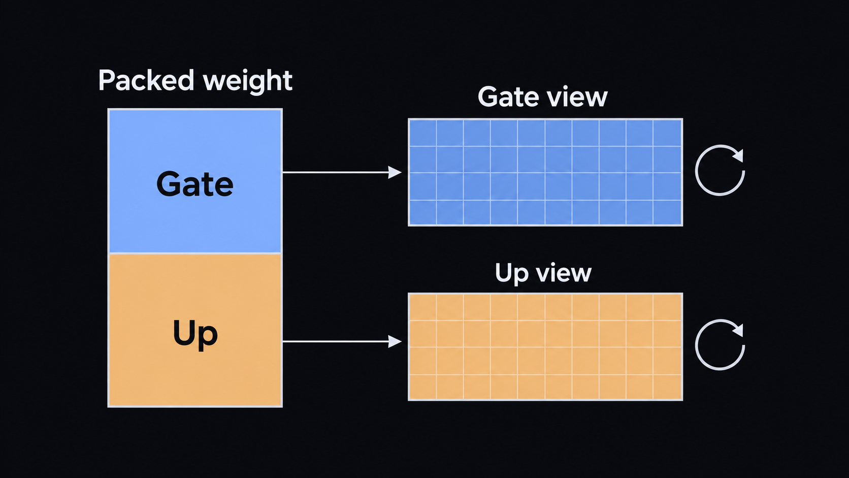
The parameter-group builder solves this with matrix views. It describes the independent pieces without replacing the original parameter or duplicating its optimizer state. For example, the actual gate/up registration is just:
_register_view(views, gate_up, (2, rows, columns))The leading 2 says that the packed parameter should be treated as two matrices, not one.
| Parameter family | Update rule | Why this grouping? |
|---|---|---|
| Hidden linear projections and expert matrices | Muon | They have a matrix update geometry. |
| Fused FFN gate/up, KDA Q/K/V and selected MLA head projections | Muon on independent views | Storage combines projections or heads that should be transformed separately. |
| Embeddings, output classifier, normalization, gates represented as vectors and depthwise filters | AdamW | They should not be forced into the same matrix orthogonalization rule. |
There is one extra detail for MLA. The head-wise K/V up-projection contains key and value rows with different roles, so its Muon view separates those rows too. The shared latent projections and output projections, by contrast, remain whole matrices. You can see the corresponding declarations in parameter_groups.py.
Every trainable parameter is assigned once. Tied embedding and output weights are deduplicated, and unselected MoE experts with no gradient are not quietly decayed. Those are implementation guarantees checked by parameter-group tests, independent-head tests and inactive-expert tests.
Even a good update needs the right pace
Choosing a direction is only half the decision. How far should the weights move at this point in training?
Imagine learning to ride a bicycle. You wouldn’t start by making your largest steering corrections at full speed. Warmup is the optimizer’s gentle start: the learning rate rises linearly over a specified number of successful updates. After that, the schedule can stay constant or follow a cosine decay toward a configured minimum fraction.
The clock is important. It counts successful optimizer updates, not attempted forwards or an arbitrary wall-clock duration. If an FP16 overflow prevents an update, training does not advance that step or the schedule. And the decay endpoint is configured independently of how many steps one particular session runs, so an interrupted run doesn’t silently get a new learning-rate curve.
The recipe tests check these boundaries. They establish the schedule’s intended arithmetic, not the best learning rate for a full pretraining run.
Keep the arithmetic and gradients under control
The parameters remain in FP32 storage. A training forward can run in FP32, BF16 or FP16 using autocast where appropriate. This gives the computation room to use lower-precision operations without converting all the long-lived weights into low precision. Selected numerically sensitive operations, including the MoE router, deliberately compute in FP32.
FP16 has a narrower usable range, so it also uses a gradient scaler. If overflow is detected, the whole hybrid optimizer update is skipped, not just Muon’s half. The next successful update still has a consistent definition. See trainer.py and the overflow test.
Before the optimizer step, the trainer also measures the global gradient norm. With max_grad_norm set to a positive value, it clips that norm if necessary. This changes an unusually large update before either optimizer handles it. With max_grad_norm: 0, clipping is disabled, although the norm is still observed.
That protects against one kind of extreme update. It does not mean every internal quantity in the model is well behaved.
QK-Clip watches a different failure mode
Attention introduces a more specific concern. Suppose the query and key vectors in an MLA head produce extremely large dot products. A global gradient norm doesn’t directly tell us how large those attention logits are.
QK-Clip watches the maximum causally valid query–key score, scaled by the square root of the query-key dimension. It combines the maxima across accumulated microbatches. If a head crosses the configured threshold, the implementation rescales selected unshared query and key projection rows after a successful optimizer update. Its shared key and value projections remain unchanged.
For a head with observed maximum and positive threshold , the rescaling factor is
A head below the threshold gets . One above it receives a factor smaller than one, distributed across the relevant projection paths. This is a weight correction informed by observed training logits, not a clamp applied to every attention score in the forward pass. Nor is it a promise that later inputs can never produce large logits. KDA’s normalized query–key mechanism isn’t a QK-Clip target here.
The behavior lives in qk_clip.py and is exercised by unit tests and training integration tests. Those tests check the defined correction and resume policy. They are not a controlled ablation proving better loss or stability.
One more kind of state: which experts learn?
In a dense layer, most parameters participate whenever the layer runs. In a sparse MoE, only the selected routed experts receive work for a given token. Quantile Balancing (QB) influences that selection using expert-specific biases. The biases affect which experts are chosen, while the mixture weights still come from the original, unbiased router scores.
Unlike model weights, QB biases are buffers, not parameters updated by Muon or AdamW. The MoE forward refreshes them in training mode. That has a surprising consequence: two gradient-accumulation microbatches are not always identical to one larger batch, because the later microbatch may encounter new routing biases. And a routed expert that received no gradient should not acquire momentum or weight decay just because other experts were active. If an FP16 update is skipped, QB may nevertheless have changed during the attempted forwards. That state is part of the training history too.
The tests check the buffer and routing distinction and bias-free mixture weighting. Whether QB improves expert utilization in a particular long run still requires run-level measurements.
A stable recipe is a testable hypothesis
The pieces now fit together. Parameter groups decide what kind of update each weight receives. Matrix views decide which directions belong together. The learning-rate schedule decides how strongly to update. Precision management, gradient clipping and QK-Clip guard different numerical failure modes. QB changes where sparse learning happens.
The repository has tests for these contracts, including Muon numerical behavior and optimizer-state continuation. I have inspected the test definitions here, not executed the suite for this chapter. They describe what the implementation is designed to preserve. They don’t establish which optimizer wins an ablation, whether clipping was necessary on a given run, or what a final pretrained model achieves.
That is the useful boundary of this chapter. The update rule is explicit enough to audit. The next question is empirical: how does that rule behave when batch size, model scale and available compute change? That’s where the scaling experiments begin.