Imagine a kitchen with dozens of chefs. Every new order could be passed to every chef, but that would be a strange way to run a restaurant. Most dishes don’t need the entire kitchen. What we want is a small team for each order, chosen according to what needs doing.
That’s the appeal of Mixture of Experts (MoE). Instead of applying one enormous feed-forward network to every token, the model has many expert networks and chooses only a few to run. More parameters can be available without paying for all of them on every token.
Of course, that creates a new problem. If we’re going to build a kitchen full of specialists, we need to decide which ones get each order, make sure their outputs behave, and stop the same two chefs from getting every single ticket. Kimi K3’s Stable LatentMoE tackles all three.
Two teams, two different jobs
Let’s follow one token through the layer. At this point, attention has already helped it gather information from other tokens. Now the model needs to transform the features inside its representation. That’s what a feed-forward network does. If you want a deeper intuition for that part, start with Dense FFN & SiTU-GLU.
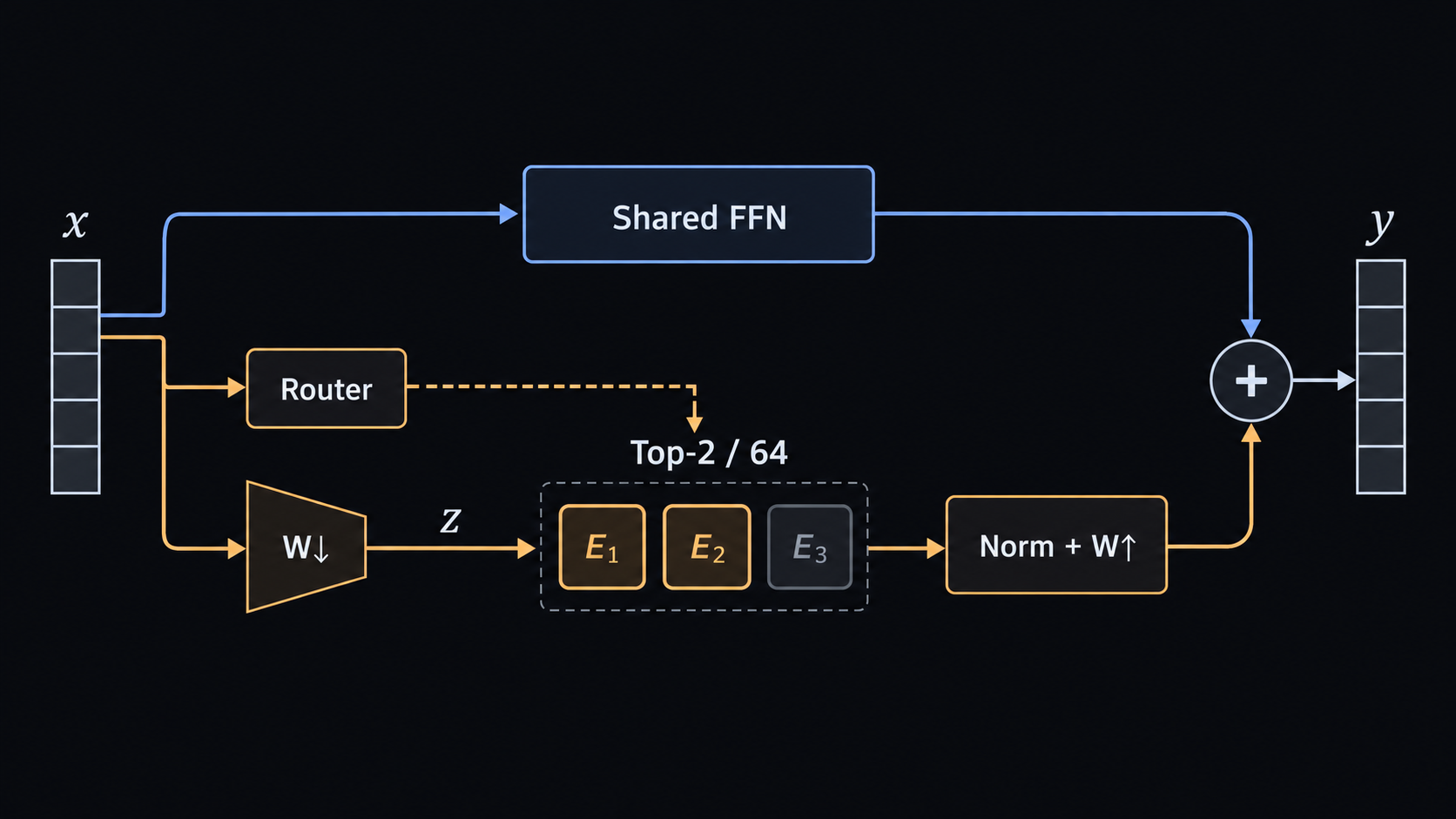
The token takes two paths at once.
One path goes to the shared experts. They run for every token, regardless of what the router decides. Think of them as the kitchen’s common prep station. They can learn transformations that are useful broadly, without having to win a competition for every order.
The other path goes to the routed experts. Here a router selects just a few candidates from a much larger pool. Different tokens can choose different experts, and the experts learn their own transformations. They aren’t labeled “grammar expert” or “math expert” in advance. Any specialization has to emerge during training.
Our smaller Kimi K3 configuration has 64 routed experts, of which 2 are selected per token, plus 2 shared experts. The original paper uses 896 routed experts and selects 16. Those numbers describe the routed pool, not the shared path. In our code, the two shared experts are implemented together as one wider DenseFFN, which is equivalent to summing separately partitioned feed-forward branches. See the model configuration and StableLatentMoE constructor.
Why send the specialists a smaller representation?
Now imagine that each specialist needs a full, bulky copy of every order. We might have saved work by calling fewer specialists, but passing around and processing all that information still gets expensive.
LatentMoE gives the routed experts a smaller working space. Before the selected experts see a token, a learned projection compresses its features into a latent vector with features. The routed experts work in that smaller space, and another projection lifts their combined answer back to the original width.
In our scaled model, that means going from 640 features down to 320, then back to 640. These aren’t necessarily human-interpretable compressed features. They’re coordinates the model learns because they’re useful for its experts.
The shared path still works directly at full width. This is an important compromise. We can make the specialized part cheaper without requiring every transformation to pass through the bottleneck.
The shape of the operation is surprisingly simple:
Read it as a journey rather than a wall of symbols. We compress the token into , let the selected specialists transform it, combine their answers into , normalize that combined answer, and return it to full width. Then we add the shared path. The paper writes the shared part as a sum of two experts. The single wider shared FFN in our reproduction implements that same kind of computation. This is the core of paper §2.3, Eq. (11).
Keeping the routed path from getting too loud
There is a catch with chaining several learned projections and expert networks. Their outputs can grow in scale. The original LatentMoE formulation could feed that varying magnitude straight into the final up-projection, where a large routed signal might overwhelm the shared one.
Kimi K3 places RMSNorm after the routed experts have been combined, but before their output is projected back up. Picture several chefs putting their contributions into one bowl. Before we send the bowl onward, we bring its overall scale back into a more predictable range. We don’t erase its direction, the pattern of features it carries. We reduce how much the size of that vector alone can dominate what follows.
The experts also use SiTU-GLU, a gated activation whose two multiplicative branches are smoothly bounded. That helps limit unusually large internal activations. The detailed gate intuition lives in the Dense FFN chapter. Here, it’s enough to see the partnership. SiTU controls what happens inside each expert, while RMSNorm controls the combined routed output between experts and the final projection.
Neither mechanism promises that training can never become unstable. They address particular ways it can become unstable. The paper’s Stable LatentMoE discussion motivates both changes, and our module places the normalization exactly at that junction.
The router makes two different decisions
We’ve talked about the selected experts as though someone simply knows which chefs to call. In practice, the router is a learned projection. For each token, it produces one score per routed expert, then passes those scores through a sigmoid. A larger score means a stronger preference for that expert.
At first, you might expect the model to pick the two largest scores and use those same numbers to mix their outputs. Mostly yes, but Kimi K3 separates two things that sound like the same thing:
- Who gets the token? The router compares scores after adding a per-expert balancing bias.
- How much does each selected expert contribute? It uses the original scores, without that bias. Our configuration then renormalizes their weights to sum to one.
This separation matters. A balancing mechanism may need to give an underused expert more chances, but that shouldn’t automatically make its answer more influential just because we needed to send it some work.
Take four experts with raw scores of 0.90, 0.80, 0.65 and 0.20. Without any adjustment, we’d choose the first two. Now suppose the first expert has been very busy and the third needs more opportunities. A selection bias of for the first expert and for the third makes their selection scores 0.50, 0.80, 0.90 and 0.20. We now choose the third and second experts.
But when we combine their outputs, we use 0.65 and 0.80, not the boosted 0.90 and 0.80. Before the routed output is normalized, their mixing weights are about 45% and 55%. The bias changed who was invited, not how much we trust the invitees’ answers. That’s the key idea behind paper §2.3.3, Eq. (13).
Quantile Balancing: giving every expert a fair shot
So how do we choose these biases? This is the part that makes the whole design feel less like a collection of tricks.
Imagine the router keeps sending most orders to a handful of chefs. Those chefs become overloaded, while others barely get any practice. In a learned MoE, that imbalance is doubly unfortunate. It can slow expert-parallel training, and an expert that almost never receives tokens gets fewer opportunities to improve.
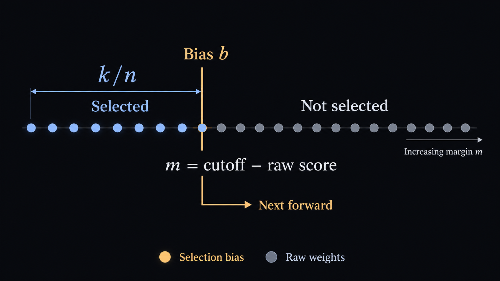
We want to balance the workload without telling the router which expert is best for a token. Kimi K3 uses Quantile Balancing (QB) to adjust the selection thresholds. The target is simple. With tokens, routed experts, and selections per token, there are expert assignments in total. A uniform load would be about assignments per expert.
Here’s the intuition. For every token, look at the expert that just missed the top-. Its score gives us a cutoff. Now examine one particular expert across all tokens. How far above or below each token’s cutoff is this expert? If we want that expert to be chosen for roughly a fraction of tokens, we can find the score threshold that puts about that fraction of its margins above the line.
That’s what a quantile gives us. Instead of nudging biases a fixed amount every time an expert is over- or underused, QB looks at the distribution of its chances of being selected and computes a new adjustment from that distribution.
In our PyTorch implementation, the essential calculation is short enough to recognize:
thresh = top_scores.view(-1, self.top_k + 1)[:, -1].unsqueeze(-1)
relative_thresh = thresh - router_scores
new_biases = torch.quantile(relative_thresh, p, dim=0, interpolation="higher")
new_biases = new_biases - new_biases.mean()
Here . thresh is the biased top- cutoff for each token. relative_thresh tells us how much extra bias each expert would need to cross that cutoff. Taking the -quantile estimates the adjustment for its target share, and centering removes an irrelevant common offset. The paper expresses the same idea using the negative -quantile of the opposite margin. The precise behavior at ties or small batches also depends on the quantile convention. See QuantileBalancer.update and paper §2.3.3, Eq. (14).
There’s a particularly nice detail. The batch chooses its experts using the old biases. The newly estimated biases are stored for the next training forward pass. Evaluation leaves them frozen. Otherwise we’d be changing the rules halfway through deciding who receives the current token.
Does QB guarantee perfectly equal loads on every batch? No. Tokens still compete for limited top- places, and finite samples, ties, and changing scores matter. QB gives the router a principled way to aim for balanced selection, not a guarantee that every expert receives exactly the same number of tokens.
The code still has to do the sparse work
There’s one last thing we shouldn’t lose sight of. Choosing two experts out of 64 saves nothing if we then run all 64 anyway.
Our StableLatentMoE implementation groups tokens by their selected expert, runs only experts that received tokens, and uses grouped matrix multiplication to evaluate them efficiently. It accumulates each expert’s weighted answer back into the right token. The simple per-expert loop remains in the file as a readable reference, while the normal forward uses the grouped path. The QB biases are buffers, not parameters updated by the gradient optimizer.
That leads to a useful distinction about evidence. The MoE unit tests are designed to check bias updates, selection versus weighting, sparse expert dispatch, normalization and gradients. The grouped-versus-naive tests compare outputs, gradients and selected-expert optimizer behavior across execution paths. These links show what is tested, not that those tests were run while writing this chapter. They also don’t demonstrate the paper’s large-scale throughput or load-balance gains in our smaller model.
We’ve arrived at a useful division of labor. Shared experts preserve a reliable full-width path. Routed experts add capacity without making every token pay for all of it. Latent projections make that route manageable, normalization and SiTU keep it better behaved, and QB helps prevent the expert pool from becoming an exclusive club.
Once we understand this, we can finally put the pieces together. In the next chapter, Backbone Assembly, we’ll see how attention, residual mixing, and this MoE layer turn a stream of token representations into a complete language model.