Dense FFN & SiTU-GLU — Kimi K3 from Scratch

Imagine you’re trying to understand the word bank in a sentence. Attention can bring you clues from nearby words like river or account. Wonderful. But collecting clues and making sense of them are not quite the same job. At some point, the model needs to take the information it has gathered and turn it into a more useful representation.

That’s where the feed-forward network, or FFN, comes in. If attention lets tokens exchange information, the FFN lets each token work on what it now knows. It applies the same learned transformation at every position, independently. No looking at neighboring tokens here. That part has already happened in attention.

The interesting question is what kind of transformation we want. Kimi K3 uses a gated FFN, with a particular activation called SiTU-GLU. To see why, let’s build it up one idea at a time.

Two views of the same information

Think of a sound mixer. One control says what signal is available. Another decides how much of that signal should come through. If we only had the first control, every signal would always contribute according to its raw strength. With two controls, the system can respond to combinations of features.

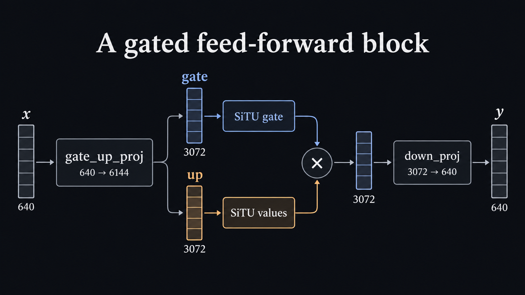
A gated FFN does something similar. It first projects a token representation into two sets of numbers. One set contains candidate values, often called the up branch. The other produces a gate, which modulates those candidates. The two branches are multiplied coordinate by coordinate, and a final projection brings the result back to the model’s original width.

\begin{aligned} g &= W_g x, & u &= W_u x, \\ z &= \operatorname{activation}(g)\odot u, & y &= W_d z. \end{aligned}

Here, $x$ is one token’s representation. $g$ and $u$ are two learned views of that same token, $\odot$ means elementwise multiplication, and $W_d$ combines the resulting features. The gate isn’t a literal on/off switch. Depending on the activation, it can smoothly amplify, suppress or even change the sign of a candidate signal.

Why bother with multiplication? Because now the contribution of one feature can depend on another. A possible interpretation of bank might matter much more when the representation also carries a strong river clue. The network learns these relationships rather than relying on a handcrafted rule.

A token representation of width 640 splits into SiTU gate and value branches of width 3072. Their elementwise product is projected back to 640 features. — **Figure 1.** A gated FFN transforms each token independently. One branch proposes values, while the other controls their contribution. Original conceptual illustration.

What happens when a signal gets very large?

A common gated FFN uses SwiGLU. Its gate is Swish, which multiplies a number by its sigmoid:

\operatorname{SwiGLU}(g,u)=(g\,\sigma(g))\odot u.

Near zero, this gives a smooth and expressive response. For a strongly negative gate, the sigmoid makes its contribution small. For a strongly positive one, the gate behaves roughly like $g$ itself.

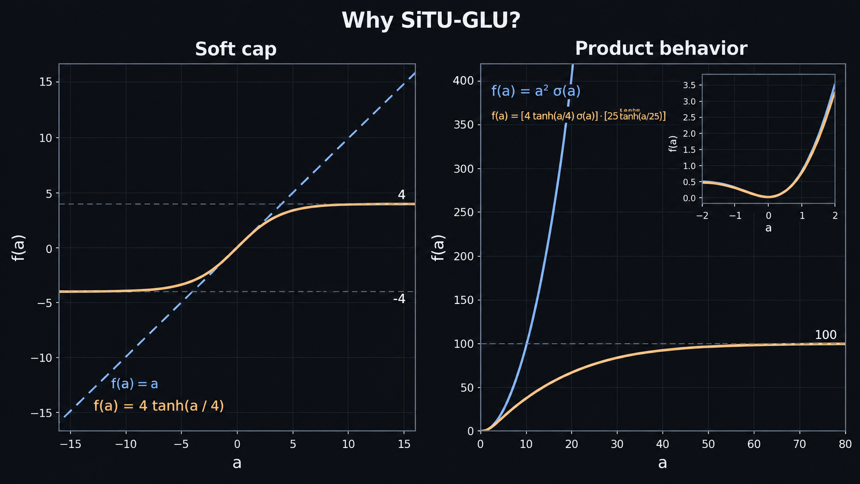
That last detail is useful, but it comes with a price. Neither the positive gate nor the up branch has a fixed bound. Imagine a coordinate where both happen to reach 100. Their product can become enormous. In a very deep or sparsely routed network, occasional large activations can make low-precision computation harder to control. Kimi K3’s paper points to this risk in its Stable LatentMoE design. Paper §2.3.2.

So why not just clamp everything to a maximum value? We could, but a hard clamp introduces a sharp boundary and a flat region beyond it. We’d like a limit that the model approaches smoothly, without abruptly changing the behavior around ordinary values.

SiTU-GLU: a soft ceiling, not a hard wall

There’s a neat function for this. Consider

\operatorname{softcap}(a,\beta)=\beta\tanh(a/\beta).

For small $a$ , it behaves almost like $a$ . Push it far in either direction and it gradually levels off near $\pm\beta$ . Think of turning up the volume on a mixer whose dial becomes progressively harder to turn near the end. There’s still a smooth response, but it can’t grow forever.

SiTU-GLU applies this soft cap to both of the factors that could otherwise become large. It retains the sigmoid part of Swish on the gate:

\begin{aligned} G(g) &= \beta_1\tanh(g/\beta_1)\,\sigma(g), \\ U(u) &= \beta_2\tanh(u/\beta_2), \\ \operatorname{SiTU\!-\!GLU}(g,u) &= G(g)\odot U(u). \end{aligned}

Read it like our mixer. The right-hand branch proposes a value, but one whose magnitude is controlled. The left-hand branch still responds to the gate and still suppresses strongly negative values through the sigmoid. Their product decides what gets passed to the down projection.

Kimi K3 uses $\beta_1=4$ and $\beta_2=25$ . Because neither bracket can exceed its respective cap in magnitude, each coordinate of the product inside SiTU-GLU has magnitude at most $4\times25=100$ . This does not bound the final output $W_d z$ , which is another learned linear transformation. Paper Eq. (12) and Appendix B.

A visual comparison would make this especially easy to see. Near the origin, the SwiGLU and SiTU responses are close. At large positive inputs, SwiGLU keeps growing while SiTU gradually levels off. This is a property of the activation, not a measured accuracy or speed improvement in our reduced model. The paper illustrates it in Figure 4.

The tanh soft cap follows the identity near zero but approaches finite limits. SwiGLU grows without bound for large positive inputs while the scalar SiTU-GLU product approaches 100. — **Figure 2.** SiTU-GLU preserves behavior near the origin while smoothly bounding its internal activation product. Analytical functions, not experimental measurements.

From the equation to our PyTorch module

Here’s the pleasant part. Our SiTU implementation looks almost exactly like the equation:

gate, values = x.float().chunk(2, dim=-1)
gate_branch = beta * torch.tanh(gate / beta) * torch.sigmoid(gate)
value_branch = linear_beta * torch.tanh(values / linear_beta)
return (gate_branch * value_branch).to(input_dtype)

The two projections are actually computed with one gate_up_proj matrix and then split in half. It’s just a convenient way to perform both projections together. In our 300M configuration, a token starts with 640 features, expands into 3,072 gate coordinates and 3,072 value coordinates, combines them using SiTU, then returns to 640 features through down_proj. The input and output widths match, even though the work happens in a wider intermediate space. Configuration.

Notice the .float() before the split. In our implementation, SiTU’s nonlinear arithmetic runs in FP32 internally, even when the incoming tensor uses BF16 or FP16, and the result is cast back at the end. That’s a deliberate numerical choice for evaluating the tanh and sigmoid operations. The module also offers an optional compiled path, but compilation isn’t part of what makes the mathematical activation SiTU.

One building block, many uses

The name Dense FFN simply means that this transformation is applied to every token in that layer. Our decoder construction uses it for the first of 13 layers. The remaining layers use Stable LatentMoE instead.

But the FFN hasn’t disappeared. In our MoE implementation, the expert transformations themselves reuse this DenseFFN and SituGLU machinery, at different widths. The distinction is which tokens are sent to which experts, not a completely different kind of nonlinear transformation. We’ll leave that routing problem to the next chapter.

Finally, how do we know the implementation matches what we’ve described? The FFN unit tests check shapes, finite outputs and gradients, the split into two branches, agreement with an explicit SiTU reference, and FP32-to-BF16 rounding behavior. Those tests check the implementation contract. They do not, by themselves, prove that SiTU improves the quality of our pretrained model, or that choosing a dense first layer is optimal.

So here’s the whole picture. Attention gathers context. The FFN transforms what each token now knows. SiTU-GLU makes that transformation expressive without allowing its internal multiplicative branches to grow without bound. That same building block will soon let us understand what an individual expert does. The next question is how to choose just a few experts for each token.