Hybrid Attention

Imagine reading a long document with a small notebook beside you. You cannot copy every sentence, so you keep updating a few useful notes. Most of the time, that’s enough. But sometimes you want to check the exact wording of something you read ten pages ago. Then a summary, however good, isn’t quite the same as having the page in front of you.

That’s the idea behind Hybrid Attention in Kimi K3. Some layers maintain a compact memory that changes as they read. Others can look directly at earlier positions in the sequence. The architecture alternates three Kimi Delta Attention (KDA) layers with one Gated Multi-head Latent Attention (MLA) layer, and adds a final MLA layer. Let’s see why those two kinds of memory make sense together. Kimi K3 paper, §2.1.

Two ways to remember what came before

With ordinary causal attention, a token can compare its query against the keys of all earlier tokens. You can think of it as keeping the earlier pages available for reference. The model doesn’t necessarily use every page, but it can decide which positions matter for the question it’s asking now.

A recurrent layer works differently. It carries a state from one token to the next, like that little notebook. The state doesn’t grow with the length of the text. That’s attractive when the sequence gets long, but there’s a catch. What should happen when the next sentence changes something we’ve already written down?

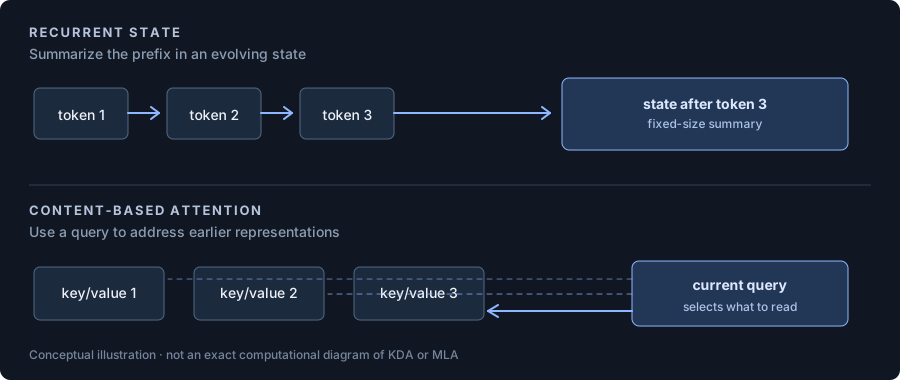
This is where KDA becomes interesting. Its memory isn’t just a running pile of information. It has a way to correct what it already believes.

KDA: don’t write the same information twice

Suppose a document says, “The meeting is on Tuesday.” A few paragraphs later, it says, “Correction: the meeting is on Thursday.” If we only kept adding new notes, we’d have both statements competing for space. What we’d really like is to update the association between this meeting and its date.

KDA does something analogous, using vectors rather than literal notes. Each attention head carries a matrix $S_t$ that acts like a small, learned associative memory. A key $k_t$ tells it which association the current token addresses. A value $v_t$ says what that association should return. A query $q_t$ lets the model read from the resulting memory.

The clever step comes before writing. KDA asks the memory what it would already return for the new key. It then writes only the difference between that prediction and the new value.

For now, ignore forgetting. If the memory predicts a value of 2, but the new information says 6, the difference is 4. With a write strength of 0.5, the prediction moves halfway toward 6, ending at 4. With a normalized key, that’s exactly how the delta update behaves along that key direction. The model doesn’t have to learn the same association from scratch every time.

Here’s that idea in mathematical form, including KDA’s forgetting step:

You can read this from left to right. $M_t$ is the memory after retaining some of the past. $\widehat{v}_t$ is its current answer for key $k_t$. The difference $v_t-\widehat{v}_t$ is what needs correcting. The factor $\beta_t$ decides how strongly to make that correction. Once the memory is updated, the query reads from $S_t$.

Notice the important part: if the memory already gives the right answer, there is nothing to correct. That’s why the subtraction is there. This is the delta rule, expressed in the state orientation used by our code. It’s algebraically equivalent to Kimi K3, §2.1.1, Eq. (1).

The recurrent PyTorch implementation follows this story almost line for line:

S = alpha_t * S                 # Retain what matters
v_old = torch.einsum("bhkv,bhk->bhv", S, k_t)
delta_v = v_t - v_old           # What did memory get wrong?
S = S + beta_t * (k_t.unsqueeze(-1) * delta_v.unsqueeze(-2))

In the full module, short causal convolutions first give Q, K and V a little local context. The implementation normalizes queries and keys, scales the readout, and learns an output gate to control which channels are passed onward. The memory correction is the central idea, not the entirety of the layer.

Forgetting can be selective, too

Let’s go back to the notebook. Not all notes deserve the same lifespan. A temporary detail might stop being useful quickly, while the main subject of a document could stay relevant for hundreds of tokens.

Earlier gated delta mechanisms can decay an entire head’s memory by one scalar. KDA instead uses a vector of retention factors $\alpha_t$. Each factor scales a different key channel of the memory. In other words, the model can keep some directions strongly while letting others fade.

For example, retention factors of 0.95 and 0.10 would preserve most of one channel while discarding most of another. These channels are learned coordinates, not dedicated slots for individual facts. That’s an important distinction, but the intuition holds: forgetting need not happen at the same speed everywhere.

KDA also bounds its log-decay, which helps make the parallel calculation numerically manageable. Our scaled configuration uses a lower bound of $-5$, following the mechanism in the paper. Kimi K3, §2.1.1.

But isn’t a recurrent update sequential?

Yes, at least in the way we’ve described it so far. Token 2 needs the memory left by token 1, and token 3 needs the memory left by token 2. That makes the recurrence easy to understand, but a poor fit for training on a GPU if we naively process every token one at a time.

Here’s the useful twist. We can keep the same update rule while changing how we compute it. The chunkwise PyTorch version groups tokens, works out their causal dependencies through a triangular solve, and passes the memory between chunks. Our tests compare its outputs and gradients with the simple recurrent version.

The readable chunkwise implementation requires sequence lengths divisible by the chosen chunk size. For the larger training setup, the repository can alternatively call an optimized FLA Triton kernel. That fused kernel is externally provided, not part of our original PyTorch derivation. The algebra behind the chunkwise transformation deserves a longer article. For understanding Hybrid Attention, what matters is that parallel execution doesn’t require changing the memory we want to compute.

MLA: sometimes you want to look at the page again

Even a very good notebook has a limitation. It compresses what you’ve read. If two distant passages contain subtly different information, a compact memory has no guarantee of preserving both exactly. Sometimes it’s valuable to compare the current token with distinct earlier positions instead.

That’s the job of the occasional Gated MLA layer. It uses causal softmax attention, so a query can still assign different attention weights to earlier positions. The difference from ordinary multi-head attention is how the information used by the heads is represented.

Rather than constructing every head’s keys and values straight from the full hidden state, MLA first creates a smaller latent representation. Head-specific keys and values are then reconstructed from that latent. Think of it as storing a compact description of each page while still keeping the pages separate. We haven’t collapsed the whole document into one recurrent memory.

Our implementation has another interesting detail. Each key combines a head-specific content part with a shared part seen by all heads. The code makes these steps visible in GatedMLA, followed by PyTorch’s causal scaled dot-product attention.

The paper’s MLA also uses No Position Encoding (NoPE). These layers do not add RoPE to their queries and keys. That doesn’t mean the full backbone ignores token order. The surrounding KDA layers already mix information through causal convolutions and recurrent updates. Finally, a learned output gate controls which attention output channels reach the rest of the network. Kimi K3, §2.1.2.

One boundary is worth keeping clear. The paper discusses caching compressed latent representations during inference. Our reference GatedMLA.forward performs the attention computation but does not implement a persistent KV cache. And unlike KDA’s fixed-size recurrent state, global MLA still attends across earlier positions.

Why alternate them?

Now the pattern feels less arbitrary. Most layers work with a compact memory that can forget and correct itself. Periodically, a global attention layer can reach directly across the available prefix. KDA gives the model an economical way to keep updating its past. MLA provides a different way to consult it.

In our 13-layer scaled configuration, layers 1–3, 5–7, and 9–11 use KDA. Layers 4, 8, and 12 use MLA, with a final MLA at layer 13. This preserves the paper’s pattern at a much smaller scale, not its full model size or capabilities.

The code selects the mechanism through layer_types in the decoder block. The KDA tests check correspondence between the recurrent and chunkwise implementations, while the MLA tests compare the module with an explicit attention reference. The integration tests cover assembly. Those are references to implemented tests, not a claim that they were executed for this editorial revision.

So we arrive at a useful division of labor. KDA keeps revising a compact memory. MLA can revisit individual positions. Together, they give the backbone two complementary ways to use the past. Next, we’ll look at a different question: how information moves between the layers themselves.